Key Performance Metrics
📊 How Well Does This Strategy/Model Perform?
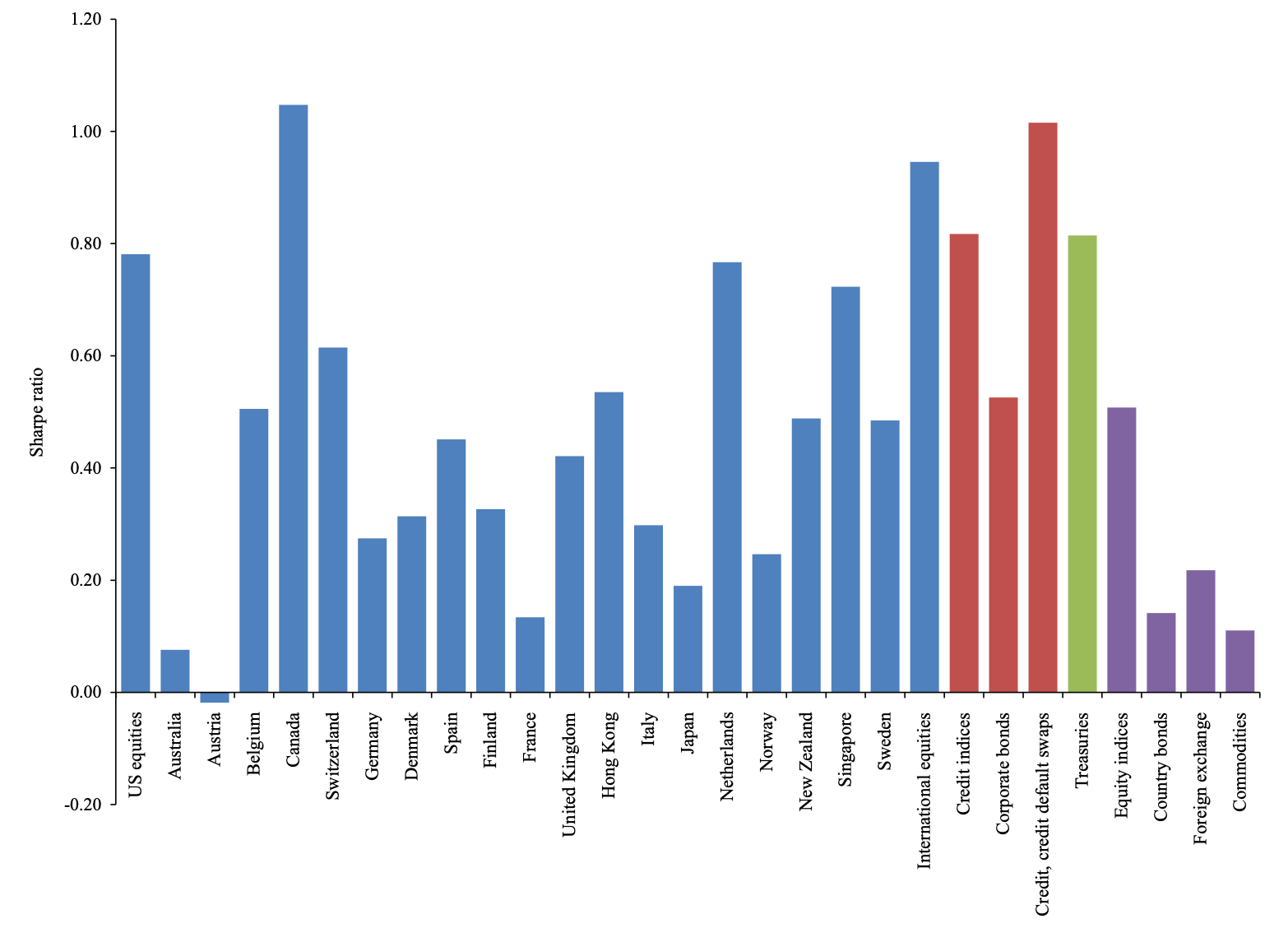
- US Stocks Sharpe Ratio (BAB Factor): 0.78
- Treasury BAB Sharpe Ratio: 0.81
- Corporate Credit BAB Sharpe Ratio: 0.82
- Alpha: Significant in 18 of 19 developed equity markets
💡 Takeaway:
Betting against beta delivers strong, positive, and consistent returns across time, countries, and asset classes—outperforming traditional equity factors like value and momentum.
Key Idea: What Is This Paper About?
The paper explains why low-beta assets outperform on a risk-adjusted basis. Investors who can’t use leverage are forced to chase high-beta assets for higher expected returns, pushing their prices up and expected returns down. In contrast, low-beta assets are underpriced. A market-neutral portfolio that goes long low-beta assets (leveraged) and shorts high-beta assets earns high returns.
Economic Rationale: Why Should This Work?
📌 Relevant Economic Theories and Justifications:
- Leverage Constraints: Investors unable to borrow overweight risky (high-beta) assets instead of leveraging safer ones.
- Flattened Security Market Line: When many agents are constrained, the CAPM becomes too flat—high-beta assets have lower alpha.
- Funding Liquidity Risk: When liquidity tightens, the BAB strategy suffers short-term losses but earns higher returns afterward.
- Market Clearing Mechanism: Unconstrained investors arbitrage by leveraging low-beta assets and shorting overpriced high-beta ones.
📌 Why It Matters:
It challenges the classic CAPM and redefines the role of leverage and risk-taking in asset pricing. The results reshape portfolio construction and performance attribution.
How to Do It: Data, Model, and Strategy Implementation
Data Used
- Asset Classes: US & international equities, Treasuries, corporate bonds, credit indices, FX, commodities
- Period: US equities from 1926, global from 1980s, others vary (1950s–2012)
- Sources: CRSP, MSCI, Xpressfeed, Barclays Bond Hub, AQR internal data
Model / Methodology
- Key Model Feature: Multiple investor types with different leverage constraints and risk aversion
- BAB Construction:
- Sort assets by beta
- Go long low-beta assets (leveraged to beta=1)
- Short high-beta assets (de-leveraged to beta=1)
- Result: Market-neutral portfolio capturing the beta anomaly
Trading Strategy (BAB Factor)
- Signal Generation: Use historical rolling beta to sort assets
- Portfolio Construction:
- Long side: leverage low-beta assets
- Short side: de-leverage high-beta assets
- Rebalancing: Monthly
- Risk Targeting: Equal beta exposure long and short, volatility-scaled
Key Table or Figure from the Paper

📌 Explanation:
- Plots annualized Sharpe ratios of BAB strategies across stocks, bonds, credit, FX, and commodities
- Almost all asset classes show positive Sharpe ratios, with US stocks and Treasuries exceeding 0.80
- Highlights the consistency and robustness of the BAB effect across global markets and asset types
Final Thought
💡 You don’t need to take more risk to earn more—you just need to bet against beta. 🚀
Paper Details (For Further Reading)
- Title: Betting Against Beta
- Authors: Andrea Frazzini, Lasse Heje Pedersen
- Publication Year: 2014
- Journal/Source: Journal of Financial Economics
- Link: https://doi.org/10.1016/j.jfineco.2013.10.005
