💡 Takeaway:
The GAN-based SDF model dominates benchmarks across every asset pricing metric—explaining more return variation, capturing more pricing anomalies, and generating higher Sharpe ratios with lower risk.
Key Performance Metrics
- Out-of-Sample Annual Sharpe Ratio: 2.6 (GAN) vs. 0.8 (FF5), 1.7 (linear GAN), 1.5 (FFN)
- Explained Return Variation (Individual Stocks): 8%
- Cross-Sectional R²: 23%
- Explained Variation on Anomaly Portfolios: >90% on all 46 decile sorts
- Robust to Size Restrictions: Sharpe Ratio = 1.4 on top 1,500 stocks
Key Idea: What Is This Paper About?
The paper estimates the stochastic discount factor (SDF) for all U.S. equities using a deep learning asset pricing model. It combines three neural network architectures:
- A feedforward network to model non-linear interactions,
- An LSTM to extract macroeconomic hidden states,
- A GAN to select the most informative pricing moments.
By embedding no-arbitrage constraints into the training, the model avoids overfitting and delivers strong pricing performance both in- and out-of-sample.
Economic Rationale: Why Should This Work?
📌 Relevant Economic Theories and Justifications:
- No-Arbitrage Pricing: SDF is estimated via conditional moment constraints across all assets.
- Machine Learning as General GMM: GAN selects the most mispriced portfolios for moment enforcement.
- Heterogeneous Risk Premia: Risk loadings (βs) vary non-linearly with characteristics and macroeconomic states.
- Time-Varying Dynamics: LSTMs learn economic regimes (booms/recessions) from macro data instead of using lagged variables or differences.
📌 Why It Matters:
This approach integrates machine learning into asset pricing without discarding economic structure, offering interpretable, testable, and practically useful models.
How to Do It: Data, Model, and Strategy Implementation
Data Used
- Returns: Monthly stock returns from CRSP (1967–2016)
- Characteristics: 46 firm-specific predictors
- Macro Data: 178 time series from FRED, Compustat, and Welch-Goyal
- Assets: 10,000+ stocks, 46 anomaly portfolios
Model / Methodology
- SDF Estimation:
- GAN solves a minimax game: minimize pricing errors across all stocks vs. maximize pricing failure across conditions
- Architecture:
- Feedforward Network (SDF weights ω)
- LSTM (macroeconomic hidden states)
- GAN (moment condition selection)
- Comparison Benchmarks:
- FFN (simple deep learner), EN (elastic net), LS (linear special case), FF3 and FF5
Trading Strategy (From SDF Output)
- Signal Generation:
- Use GAN-estimated risk loadings (β) to sort stocks
- Long high-β (high SDF exposure), short low-β
- Portfolio:
- Mean-variance efficient SDF portfolio
- Rebalance monthly
- Risk Metrics:
- Max drawdown, turnover, max loss compared across models
Key Table or Figure from the Paper
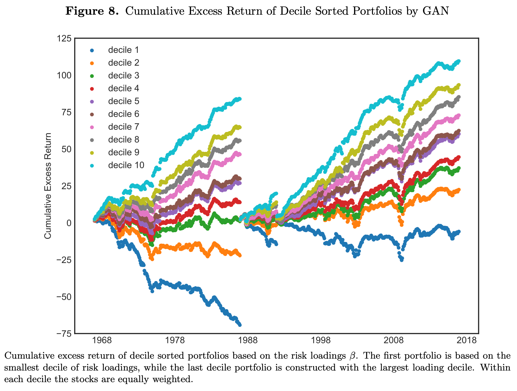
📊 Reference: [Figure 8] – Cumulative Return of β-Sorted Portfolios (Test Sample)

📌 Explanation:
- Stocks sorted by GAN-estimated β loadings produce monotonic return patterns.
- Top decile outperforms bottom decile by 48% per year.
- None of the Fama-French factors explain the return spread—GRS test strongly rejects.
- This validates that the GAN model captures systematic pricing risks.
Final Thought
💡 Deep learning with economic discipline solves asset pricing better than ever before. 🧠📈
Paper Details (For Further Reading)
- Title: Deep Learning in Asset Pricing
- Authors: Luyang Chen, Markus Pelger, Jason Zhu
- Publication Year: 2019
- Journal/Source: SSRN Working Paper
- Link: https://ssrn.com/abstract=3350138
