💡 Takeaway:
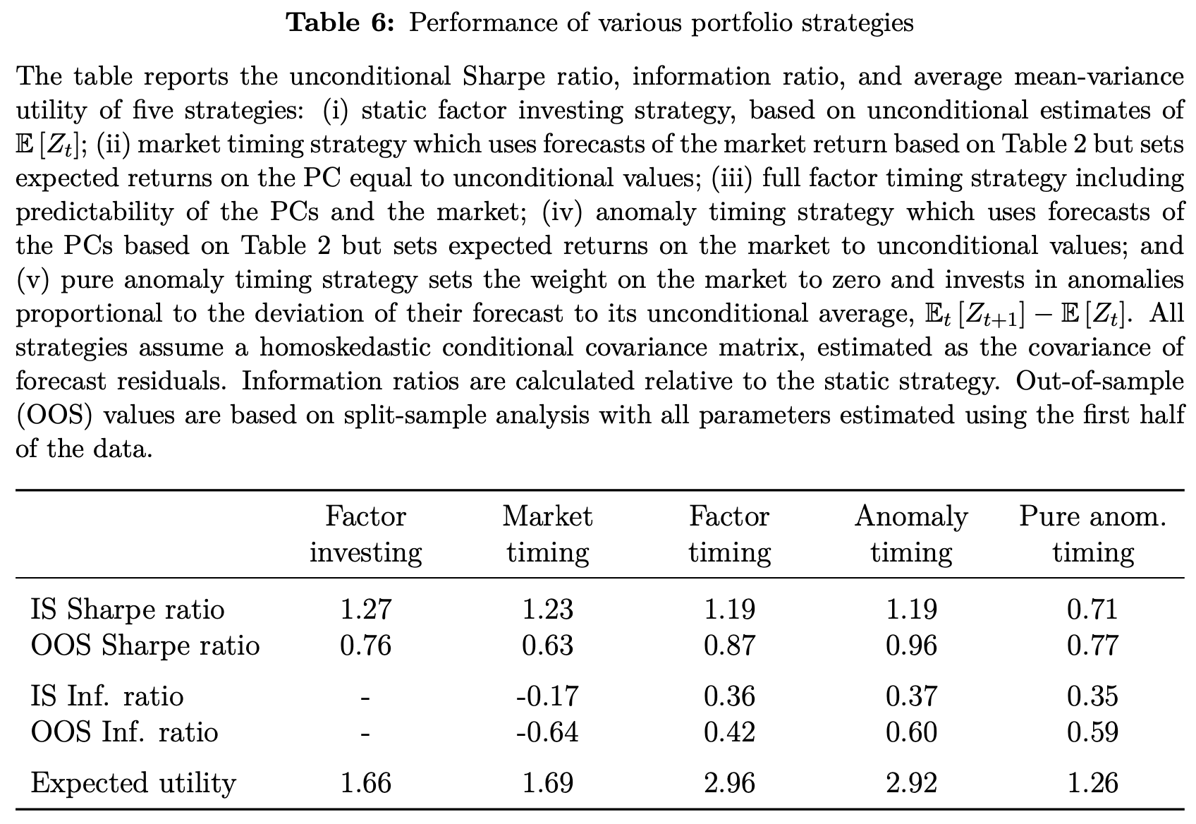
Factor timing leads to meaningful gains, doubling utility compared to static factor investing and outperforming pure market timing strategies.
Key Performance Metrics
📊 How Well Does This Strategy/Model Perform?
- Sharpe Ratio (Out-of-Sample):
- Static Factor Investing: 0.76
- Full Factor Timing: 0.87
- Pure Anomaly Timing: 0.77
- Monthly Alpha (Composite Mood Beta Portfolios): Up to 2.37%
- SDF Variance: Increases from 1.67 (static) to 2.96 (timing)
Key Idea: What Is This Paper About?
This paper introduces a method for timing equity factor exposures using valuation ratios (like book-to-market) to predict future returns of principal components (PCs) of anomaly portfolios. By forecasting only the most important factors (top 5 PCs), they reduce noise and avoid overfitting. The resulting portfolio strategy earns superior risk-adjusted returns and reveals that the true stochastic discount factor (SDF) is more volatile and dynamic than previously thought.
Economic Rationale: Why Should This Work?
📌 Relevant Economic Theories and Justifications:
- Time-Varying Risk Premia: Expected returns on equity factors change over time with macro cycles and investor preferences.
- No Near-Arbitrage Principle: Without excessive Sharpe ratios, only dominant components (large PCs) of factor returns should be predictable.
- Dimensionality Reduction (PCA): Predicting a few key PCs avoids noise and identifies common sources of factor return dynamics.
📌 Why It Matters:
These findings challenge traditional asset pricing models, suggesting that multiple, time-varying sources of risk premia drive returns, not a single market factor.
How to Do It: Data, Model, and Strategy Implementation
Data Used
- Assets: 50 equity anomaly portfolios (e.g., value, size, momentum)
- Time Period: 1974–2017
- Source: CRSP, COMPUSTAT
- Predictors: Portfolio-level book-to-market ratios
Model / Methodology
- Use Principal Components Analysis (PCA) to reduce 50 anomalies to top 5 PCs
- Forecast each PC using its own valuation ratio (bm)
- Use out-of-sample (OOS) validation and placebo tests to ensure robustness
- Construct Stochastic Discount Factor (SDF) from predicted PC returns
Trading Strategy
- Signal Generation:
- Predict top 5 PC returns monthly using each PC’s valuation ratio
- Portfolio Construction:
- Long-short strategy: Overweight PCs with higher expected returns
- Include or exclude market exposure depending on version (pure anomaly vs. full timing)
- Rebalancing: Monthly (robust to lower frequencies like quarterly/annual)
Key Table or Figure from the Paper

📌 Explanation:
- Shows performance of five portfolio variants (static, market timing, factor timing, anomaly timing, pure anomaly timing)
- Full factor timing portfolio earns the highest Sharpe (0.87 OOS) and expected utility
- Timing only anomalies yields 0.77 OOS Sharpe—higher than market timing (0.63)
Final Thought
💡 You don’t need to time the market. Timing factor exposures can deliver stronger and more consistent alpha. 🚀
Paper Details (For Further Reading)
- Title: Factor Timing
- Authors: Valentin Haddad, Serhiy Kozak, Shrihari Santosh
- Publication Year: 2020
- Journal/Source: NBER Working Paper No. 26708
- Link: https://www.nber.org/papers/w26708
